|
|
|
Definition.
 | Cost are expenses or
expenditures by the firm in the process of producing goods and services. |
 | Cost refers to the
expenditure incurred by the firm in producing output or incurred in the process
of consuming goods and services. |
Therefore cost refers to the money outlay (income) used to
purchase factors of productions. |
|
There are
mainly four types of costs:
 | 1. Opportunity cost |
 | 2. Social cost |
 | 3. Private cost |
 | 4. Fixed and variable costs |
|
|
1.
OPPORTUNITY COST:
Opportunity
cost refers to the real cost of obtaining something. It involves sacrification.
It is not a monetary cost but sacrification
-
Opportunity cost refers to the alternative that must be forgone or sacrified
when the second alternative is selected
Eg. The
consumer decides to hire house instead of a car since his income is not enough
to purchase both (Opportunity cost is that alternative forgone (car)
(In
detail refers pp and isoquant curve)
IMPORTANCE
OF OPPORTUNITY COST
 | It is used to determine
decision on resource allocation
(Ref: ppc) |
 | It is used to determine the
price in the market (Price determination) eg consumer substitute commodity which
it has low price eg consumer substitute goods which has low price. |
 | It is used to determine how
much will be consumed and how much will be produced. |
|
|
2.
SOCIAL COST (COLLECTIVE COSTS)
Social
cost refers to cost owned by the society in the whole process of civilizing
public goods.
Eg:
Expenses on education, health services, transpotation, communication etc
. |
|
3.
PRIVATE COST PUBLIC
Private
cost are expenses or expenditure incurred by the individuals (firms, industry)
in the process of producing goods and services since the level of production
differ from one firm to another.
TYPES
OF PRIVATE COSTS
 | i.
Implicity costs (imputed costs) (pocket) |
 | ii.
Explicit cost (out pocket cost. |
i.
IMPLICITY COST:
Implicity
costs are self-owned are pocket cost or pocket cost. These are self owned costs
or self owned resources incurred by the firm or an industry the process of
producing output or sometimes called opportunity cost of business operation (sacrification
costs) eg salary of the owner and manager who only receive profits.
-
eg estimated rent for his building are implicit costs. These are not
estimated or counted.
ii.
EXPLICITY COSTS.
Explicit
cost refers to costs that the firm or an Industry incurred in the process of hiring
factors of production.
-
All expenses used to hire factors of production.
Eg purchasing raw materials.
-
Paying worker’s wage.
-
Rented charges
-
Interest etc.
|
|
TOTAL
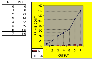
VARIABLE COST (TVC)
Tvc refers to prime costs. These are which do vary with
output, cost which change at any level of output, eg cost on raw materials,
labour expenses, cost of power, fuel, maintenance, repair etc. These costs,
don’t exist if output is zero
 Q
= f (TVC) Q
= f (TVC)
|
|
In short
run production function is given by Q= f (L,Te) TVC= PL-L
Where
PL = Price of variable input.
L = number of variable input.
Example:
A firm employs 10 workers at average of 20,000/- calculate TVC of the firm.
Sol:
PL = 20,000
L = 10 workers
TVC = PL.L
= 20,000*10
TVC
= 200,000
NB.TVC exist in short run and long run period
* TVC
don’t exist if Q=0
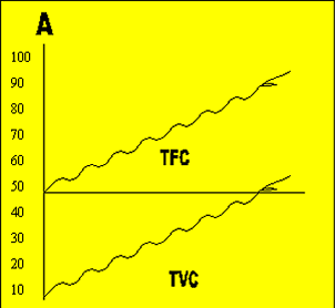
From the diagram above
at (0) level of output,
TC = TFC = 50 since when Q=0,TVC=0
As production commences
the firms hires only variable factors hence the shape of TC will depend on the
behavior of TVC since change in output will depend on TVC.
Q =
f(TVC)
TC = f(Q)
QUESTION: Account for the TC at
zero level of output.
Solution:
At zero level of output TC=TFC
Since TVC=0
When production
commences the shape of TC will be determined by the behaviour of TVC since
2 = f(TVC)
TC = f(Q)
|
|
THE RELATIONSHIP BETWEEN
AVERAGE FIXED COST,
AVERAGE VARIABLE COST,
AVERAGE COST AND MAGINAL COST IN SHORT RUN PERIOD.
|
AVERAGE
FIXED COST: (AFC)
AFC
refers to fixed cost per unit of output.
AFC is the ratio between Total fixed cost and the level of output.
AFC=TFC/Q
The short
run period production function is given by.
Q= f(lk)
TFC = PK * K
AFC = PK *K /Q
AFC = PK * K /Q - i
AFC = TFC / Q - ii |
Explicity
cost are cost called pocket costs. These cost must be estimated or accounted in order to determine the losses or
profits of the firm.
|
|
IV)
TOTAL FIXED COST AND VARIABLE COST (TFC)
TOTAL FIXED COSTS (TFC)
TFC
refers to that costs which don’t vary with the level of output. It means
always remain constant at any level of production (OUTPUT).
TFC are also called overhead costs or supplementary costs
These
costs exist even if firm produces nothing.
1.
When Q = 0 TFC exists 2.
Exist in only short run
| Q |
TFC |
*TFC curve remain
constant
- Examples of fixed
costs
- Purchase of machines, a
piece of land
|
| 0 |
20 |
| 1 |
20 |
| 2 |
20 |
| 3 |
20 |
| 4 |
20 |
| 5 |
20 |
In
shorten Production function is given by
Q = f(l,k)
TFC = Pk x k
Where
Pk = Price of fixed factor
k = Unit of fixed input
Question
Example: A firm produced a machinery
which costs 200,000 Tshs Calculate TFC
Solution
Given k = 1
P = 200,000/Tshs
TFC
= Pk x k
TFC
= 200,000 x 1
AVC =
PL.L /Q
AVC = TVC / Q
| Q |
TVC |
AVC |
 |
| 0 |
0 |
- |
| 1 |
18 |
18 |
| 2 |
30 |
15 |
| 3 |
40 |
133 |
| 4 |
52 |
13 |
| 5 |
65 |
13 |
| 6 |
82 |
13.7 |
| 7 |
106 |
15.14 |
|
|
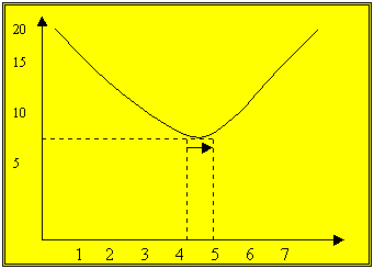
The
behavior of AVC Curve is U-Shaped.
Initially falls reached at a minimum point then starts to rise as output is
expanded.
The U Shaped of AVC curve is due to returns to scale or Economies and di-economics
of scale.
Due to internal economies of scale reached at minimum and then start rising as
diseconomies of scale.
|
|
AVERAGE
TOTAL COST OR AVERAGE COST (AC)
AC refers
to TC per Unit of output
AC refers to the ratio between TC and the level of output
AC = TC
/Q
Since
Q = f ( l,k )
TFC
= Pk.k
TVC
= PL.L
AC = Pk.k + PLxL /Q
TOTAL
COST (TC)
TC refers to the sum of TFC and TVC
TC = TFC + TVC
Where
TC = Total cost
TFC = Total Fixed Cost
TVC = Total Variable Cost
Since in short run period production is
given by
Q = f ( L,k )
TFC = Pk x k
TVC = PLx L
TC = Pk x k + PL* L
TC= TFC + TVC
Note:
since the change in the level of output depends on TVC, therefore TC is function
of output;
TC = F (Q)
Q = F(TVC)
When
Q = 0 TVC = 0
and TC =TFC
The Summary
TC = Pk.k + Pk.L
TC = TFC + TVC
TC = f(Q)
| Q |
TFC |
TVC |
TC |
 |
| 0 |
50 |
0 |
50 |
| 1 |
50 |
15 |
65 |
| 2 |
50 |
25 |
75 |
| 3 |
50 |
34 |
84 |
| 4 |
50 |
42 |
92 |
| 5 |
50 |
52 |
102 |
| 6 |
50 |
64 |
114 |
|
|
MARGINAL
COST (MC)
MC refers
to the rate of change of TC with a given one unit.
MC refers to an increment of TC as the result of one more unit change in output.
MC refers to an additional TC with a given one more unit change in output.
MC = 4TC
/ 4Q
Since 4TC = TC2 - TC1
4Q = Q2 - Q1
MC
= TC2 - TC1 / Q2
- Q1 = 4TC / 4Q
MC= 4TC / 4Q |
| Q |
TC |
MC |
|
| 0 |
20 |
- |
| 1 |
38 |
18 |
| 2 |
50 |
12 |
| 3 |
60 |
10 |
| 4 |
72 |
12 |
| 5 |
85 |
13 |
| 6 |
102 |
17 |
| 7 |
126 |
24 |
| 8 |
160 |
34 |
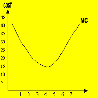
MC curve
is U-shaped due to the low of variable propotions.
MC curve initially falls reached at a minimum then start to rise as output is expanded.
| Q |
TFC |
AFC |
|
| 0 |
50 |
- |
| 1 |
50 |
50 |
| 2 |
50 |
25 |
| 3 |
50 |
18.6 |
| 4 |
50 |
12.5 |
| 5 |
50 |
10 |
| 6 |
50 |
8.3 |
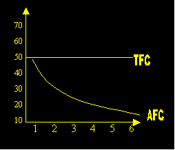
The shape
of AFC curve is that of rectangular Hyperbola
always is down ward shoping (negatively
sloped ).
A decreases as the level of output increases but will never be eg to zero.
ie. touch the x-axis
- When Q becomes
large and larger the values of AFC becomes smaller and
smaller.
- When devide a number which is fixed with a number which is variable the values of AFC
becomes smaller AFC is always positive .
AFC = TFC
/ Q
|
|
AVERAGE
VARIABLE COST (AVC)
AVC
refers to the variable cost per unit of output.
AVC is the ratio between TVC and
the level or units of output .
AVC = TVC /
Q
Since
Q = f (L,k)
TVC = PL,L
AVC
= PL,L / Q
AVC
= PL,L
/ Q
|
|
IMPORTANCE
OF AVC, AC AND MC
A. IMPORTANCE OF AVC
 | AVC is used to type of production technique used in
production of goods and services. |
 |
Whether the fom can adopt capital intensive
or labor-intensive technique will depend on costs of employing variable factors
Q= F(TVC). |
B.
AVERAGE COST (AC)
 |
Ac is used to dertemined the loses and
profits of the firm during production process |
TC = TFC + TVC
AC = TRC/Q + TVC /Q
AC = AFC +
AVC
C. MARGINAL COST ( MG)
 |
Marginal cost is used to detemine whether
the firm will expand its production, remain in production or quit
production |
 |
Mc used to
determine if the firm will embark with
large scale production or not.
|
 |
QUESTION
An: Average cost
function of a firm is given by
AC = 2Q+6+13/Q |
 |
Required:
(i) Determine fixed cost of the firm.
(ii) Determine variable cost of the form.
(iii) If the firm produces 15 units of output dertemined the effects of the
three units decrease in output. |
AC = Pk.k / Q + PL.L / Q
Ac = AFC +AVC
AC = TC /Q
AC = AFC + AVC
| Q |
TFC |
TVC |
TC |
AFC |
AVC |
AC |
MC |
| 0 |
20 |
0 |
20 |
- |
- |
|
|
| 1 |
20 |
18 |
38 |
20 |
18 |
|
|
| 2 |
20 |
30 |
50 |
10 |
15 |
|
|
| 3 |
20 |
40 |
60 |
6.05 |
18.5 |
|
|
| 4 |
20 |
52 |
72 |
5 |
|
|
|
| 5 |
20 |
65 |
85 |
4 |
|
|
|
| 6 |
20 |
82 |
102 |
3.33 |
|
|
|
| 7 |
20 |
106 |
126 |
2.86 |
|
|
|
| 8 |
20 |
140 |
160 |
2.5 |
|
|
|
|
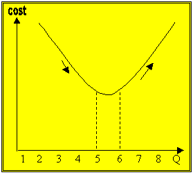 |
-AC Curve is U-shaped due to the level of variable proportions (return to scale)
-AC
Curve initially fall, reached at a minimum point then start to rise as output is
expanded |
|
|
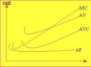
i.
Initially AFC AVC, AC and me Curve fall simultaneously
ii. MC Curve reached at minimum point still AFC, AVC and AC are falling
iii. Mc start to rise white AFC,
AVC and ac curves are still falling
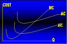
iv. AC curve intersects with mc curve when ac curve is at minimum and mc
curve is rising.
- Likewise AVC curve intersects with mc curve
when AVC curve is at minimum and mc curve is rising.
- AFC curve is down ward sloping ( it is continuously falling). |
|
|
Note: when
MC, AVC and AC curves are falling, always MC, AVC and AC curves is below and AVC
and AC (MCL, AVC and MC, LAC )
Why??.
When cast fall, are falling at small rate hence the adition
of TC become smaller than AC and AVC
*When MC, AVC and AC curve rise always MC
curve is above AVC and AC (MC > AC, MC > AVC)
* When cost rise, they rise at faster rate
hence the additional cost become larger than AVC and AC values.
Some points to be noted.
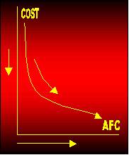
Why AFC curve is down wards sloping.
*When divide fixed costs with output which tend to change with time the values
of AFC become smaller and smaller (rectangle hyperbola)
 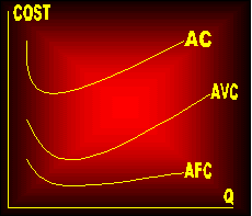
Why: AC curve is
above AFC and AVC curves.
 |
The behaviour of
ac curve will depend on the behaviour of AFC and AVC. |
 |
AC is higher than
AFC and AVC due to the reason that A
AC
= AFC + AVC |
 |
AVC is sub set of
AC. |
 |
AFC “
“ “
“ AC. |
AC > AFC
AC > AVC
WHY
AVC, AC AND, MC ARE U-SHAPED IN SHORT RUN
Why
AVC is u-shaped in short run :
METHOD
I:
The u-shaped of AVC curve be explained by using the relationship
between APL and AVC
TVC =PL.I
Where:
TVC = total variable cost
PL = Price of variable input e.g. wage (w)
L = No of labour, workers employed by the firm
TVC = PL.L . . . (I),
Since PL = W
TVC = W . L . . . (II)
AVC = TVC / Q . .
. (III)
Since TVC = W.L
AVC = W.L / Q . . . (IV)
AVC = W.L / Q . . .
(V)
But Q / L = AP
AVC = W . L / APL
AVC = W . L / APL
AVC is an inverse
or mirror reciprocal of APL
When
APL at maximum AVC of at minimum when APL falls AVC
rises
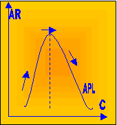 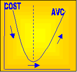
Therefore the
u-shaped of AVC is due to the behavior of APL
METHOD
II:
Method II of variable proportion.
 |
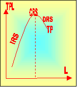
When a variable
factor (workers) are applied to fixed factor (workers) are applied to fixed
factor (a piece of land) the firm will experience. |
 |
Increase
returns to scale. |
 |
*Constant
returns to S. |
 |
*Decreasing
returns to scale. |
i.
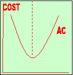
APL > AVC ---> IRS
ii. APL ~ AVC ---> CRS
iii. APL < AVC ---> DRS
Law
of Variable Proportions
The u- shaped of
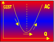
AC curve can be explained by the law of variable proportions (return to scale).
 |
i. When we add
variable factors (labour) to given number of fixed inputs e.g land the total
output will increase since cost of employing variable input is smaller than
output produced. This indicates increasing return to scale. |
 |
ii.When optimum
output is reached (TPL of max) The AC curve become at minimum hence there will
be constant returns to scale. |
 |
(iii) If the
increase in output continues beyond the optimum point the stage of diminishing
returns to scale operates and it raises the AC curve. |
WHY
MC CURVE IS U-SHAPED IN SHORT RUN
Method I: (Relationship between MC and MPL curve)
TC = TRC +TVC
MC = ATC / 4Q = A (TFC +TVC)/
4Q
MC = 4TFC + 4TVC /Q
MC = 4TFC / Q + 4TVC /Q
But ATFC = O
MC = O / 4Q + 4TVC / 4Q
MC = O + 4TVC / 4Q
MC = 4TVC / 4Q But TVC = W.L
MC = 4(W.L) / 4Q
= W.4L / 4Q Since
w is fixed
MC = W. L / MPL Since
MP = 4Q /4L
MC = W. I /
MPL
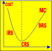
Therefore MC
curve is an inverse or reciprocal of MPL curve
 |
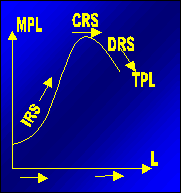
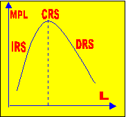
* When MPL
ases ,MC falls. |
 |
* When MPL curve
at Maximum Mc at Minimum. |
 |
* When MPL curve
falls MC ,rises. |
METHOD
III :
The Law of Variable Proportions:
 |
i. If an increase
in output is more than increase in costs of production
==>Increasing returns to scale. MPL
> MC |
 |
ii. If an
increase output is proportional to an increase in costs.
==> Constant returns to scale operates :
MPL at Maximum ~ MC at minimum |
 |
If an increase in
output is less than an increase in costs of production ==> Diminishing
returns to scale.
|
LONG RUN THEORY
OF COST
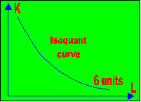 In
long run the firms are variable. All inputs are variable even those fixed inputs
existing in short run . In
long run the firms are variable. All inputs are variable even those fixed inputs
existing in short run .
In long run
production function is given by : Q
= f(c, k)
In long run in order to produce 6 units of output the firm can employ more
units of k and less units of L or more L and less k therefore in long run the
firm in curve variable costs.
LONG
RUN AVERAGE COST: LRAC
Definition
-
Long run average costs LAC refers to the small summation of Short
run average cost curve
Long run average cost curve is derived from short run
average cost curve
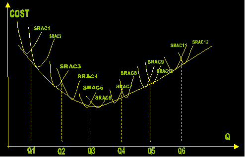
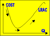 Long
run AC curve is known as planning curve or
the envelope curve since it envelopes the SAC curve. Long
run AC curve is known as planning curve or
the envelope curve since it envelopes the SAC curve.
- When the two SRAC curve intersects from one firm.-
- SRAC curves touches the longer AC curve (SRAC)curves are tanget to LR Ac
curves.
LRAC curve form an “Industry” (Small summation of SRAC curves)
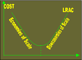
The
shape of long run curve is bowed.
*Initially LRAC curve falls reached at a minimum then start to rise.
* The shape of LRAC curve is used to determine Economies and Dis economies of
scale.
|
|
Theory
of the Cost|Types
of Cost|Opportunity
Cost|Importance
of Opportunity Cost|Social
Cost|Private
Cost|Types
of Private Cost|Total
Variable Cost|Average
Fixed Cost|Total
Fixed Cost|Average
Cost|Marginal
a \1Cost|Average
Variable Cost|Importance
of AVC,VC,MC|U-Shaped Methods
I II III
|Theory of Cost |